前言
- 这是 上一篇博客 的后续和补充,这次对边缘检测算法的升级优化,起源于一个意外事件,前一个版本是使用 TensorFlow 1.0 部署的, 并且是用 TF-Slim API 编写的代码,最近想使用 TensorFlow 1.7 重新部署一遍,本来以为是一件比较容易的事情,结果实操的时候才发现全是坑,首先遇到的就是废弃 API 的问题,TensorFlow 1.0 里面的某些 API 在 TensorFlow 1.7 里面已经是彻底废弃掉不能使用了,这个问题还好办,修改一下代码就行。后面遇到的一个问题就让我彻底傻眼了,用新的代码加载了旧的模型文件,想 Fine Tuning 一下,结果模型不收敛了,从零开始重新训练也是无法收敛,查了挺长时间也没定位到原因,所以,干脆重写一遍代码。
- 反正都要重写代码了,那也就可以把最近一年学到的新东西融合进来,就当做是效果验证了。引入这些新的技术后,原始模型其实变化挺大的,而且用到的这些技术,又会牵扯出很多比较通用的基础知识,所以从这个角度来说,这篇文章要记录的重点并不是升级优化(升级后的模型,准确性和前一个版本相比并没有明显的区别,但是模型的体积从 4.4M 减小到了 1.6M ,网络的训练过程也比之前容易了许多),而是对 多个基础知识点的梳理和总结 。
- 涉及到的知识点比较多,有工程层面的,也有理论算法层面的,和工程相关的内容会尽量用代码片段来展示,遇到理论知识,只会简单的介绍一下,划出重点,不会做数学层面的推导,同时,会在最后的『参考资料』章节中列出更多的参考内容。
- 趁这个机会也把代码重新整理了一遍,放在了 github 上,https://github.com/fengjian0106/hed-tutorial-for-document-scanning
TensorFlow Code Style For CNN Net
之前的那个版本,选用 TF-Slim API 编写代码,就是因为这套 API 是比较优雅的,比如想调用一次最基本的卷积层运算,如果直接使用 tf.nn.conv2d 的话,代码会是下面这个样子:
1 | input = ... |
如果用 TF-Slim API 编码的话,则会变成下面这种风格:
1 | input = ... |
因为在各种卷积神经网络结构中,通常都会大量的使用卷积运算,构建很多卷积层,并且使用不同的配置参数,所以很明显,TF-Slim 风格的 API 可以很优雅的简化代码。
但是,在看过图像处理领域的一些论文和各种版本的参考代码之后,发现 TF-Slim 还是有一些局限性的。常规的卷积层操作,用 TF-Slim 是可以简化代码,但是神经网络这个领域发展的速度太快了,经常都会有新的论文发表出来,也就经常会遇到一些新的 layer 结构,TF-Slim 并不是总能很方便的表达出这些 layer,因此需要一种更低层一些、但是更灵活,同时还保持优雅的解决办法。
顺着这个思路,后来发现其实 tf.layers 这个 Module 就可以很好的满足前面提到的这些需求。
另外,这次遇到的在 TensorFlow 1.7 上旧模型不收敛的情况,虽然没有准确定位到原因、没找到解决办法,但是分析了一圈后,其实还是怀疑是因为使用 TF-Slim 而引出的问题,虽然 TF-Slim 简化了卷积层相关的代码,但是完整的代码中还是要使用 TensorFlow 中的其他 API 的,TF-Slim 封装出来的抽象度比较高,除了卷积操作的 API,它还封装了其他的一些 API,但是它的抽象设计和 TensorFlow 是有一种分裂感的,混合在一起编程时会觉得有点奇怪,我这次遇到的问题,也可能就是某些 API 使用的不正确而引起的(TF1.0时运行正常,TF1.7时运行不正常)。而 tf.layers 就不会有这种感觉,tf.layers 的抽象度比 TF-Slim 更低一些,它更像是 TensorFlow 的底层 API 的一个延展,并没有引入新的抽象度,这套 API 用起来就更舒服一些。
比如,升级前的 HED 网络,换用 tf.layers 后,代码是下面这个样子:
1 | def vgg_style_hed(inputs, batch_size, is_training): |
上面这份代码里面的一些细节,会在后面的章节里详细介绍,并且会逐步的演化成 MobileNetV2 style 的 HED 网络。这里首先看一下代码的整体结构,相当于是套用了下面这种形式的模板:
1 | def xx_net(inputs, batch_size, is_training): |
这种风格的代码,前面一部分就是定义实现不同功能的各种 layer,后面部分就是用各种 layer 来组装 net 的主体结构。layer 由嵌套函数定义,方便进行各种自定义的配置或组装,net 主体部分,跟 TF-Slim 的风格其实也是类似的,layer 之间的层级关系简单明了,更容易和论文中的配置表格或结构示意图对应起来。我在实现其他网络结构的时候,都是套用的这种代码结构,基本上都能满足灵活性和简洁性的需求。
矩阵初始化
矩阵的初始化方法有很多种,在 TensorFlow 里,常规初始化方法的效果对比可以看这篇文章 Weight Initialization,能使用 tf.truncated_normal 或 tf.truncated_normal_initializer 进行初始化,说明已经对这个问题有所掌握了,随着学习的深入,更推荐使用另外一种初始化方法 Xavier initialization ,使用起来也比较简单:
1 | W = tf.get_variable('W', shape=[784, 256], |
关于 Xavier initialization 的更多内容,请参考本文末尾部分列出的资料。
Batch Normalization
Batch Normalization – Lesson 这篇教程对 Batch Normalization 解释的比较清楚,通俗点描述,普通的 Normalization 是对神经网络的输入数据做归一化处理,把输入数据和输出数据的取值都缩放到一个范围内,通常都是 0.0 ~ 1.0 这个区间,而 Batch Normalization 则是把整体的神经网络结构看成是由很多不同的 layer 组成的,对每个 layer 的输入数据再做一次规范化的操作,因为只能在训练的过程中才能获取到每个 layer 上的 input data,而训练过程又是基于 batch 的,所以叫做 Batch Normalization。Batch Normalization 的具体数学公式,这里不详细描述了,有兴趣的读者请参考末尾部分列出的资料,下面仅从工程层面提出一些建议和要注意的细节点。
Batch Normalization 的优势很明显,尽量使用
Batch Normalization 的优势挺多的,比如可以加快模型收敛的速度、可以使用较高的 learning rates、可以降低权重矩阵初始化的难度、可以提高网络的训练效果等等,总而言之,就是要尽量的使用 Batch Normalization 技术。近几年新发表的很多论文中,也是经常看到 Batch Normalization 的身影。
TensorFlow 提供了相关的 API,在 layer 中添加 Batch Normalization 也就是一行代码的事,不过因为 Batch Normalization 里面有一部分参数也是需要参与反向传播过程进行训练的,所以构造优化器的时候,还要额外添加一些代码把 Batch Normalization 的权重参数也包含进去,类似下面这样:
1 | ... |
不需要使用 bias
从前面的代码片段可以看到,用了 Batch Normalization 后,就不再需要添加 bias 偏移向量了,Can not use both bias and batch normalization in convolution layers 这里有解释原因。
在什么位置添加 Batch Normalization
前面有一个典型的代码片段:
1 | def _vgg_conv2d(inputs, filters, kernel_size): |
这里容易遇到一个陷进,我之前就掉进去过。在看其他代码和资料的时候,也经常看到 convolution + batch_normalization + relu 这种顺序的代码调用,如果理解的不透彻,很有可能会错误的认为在每一个 convolution layer 的后面都应该添加一个 tf.layers.batch_normalization 调用,但是实际上,如果当前 layer 已经是网络结构中最后的 layer 或者已经属于 output layer 了,其实是不应该再使用 Batch Normalization 的。按照定义,是在 layer 的 input 部分添加 Batch Normalization,而代码里看上去像是在 layer 的 output 上调用了一次 Batch Normalization,这只是为了在代码里让 layer 更容易连接起来,而且,如果是第一层 layer,它的输入就是已经归一化处理过的 input label 数据,这也是不需要 Batch Normalization 的,到了最后一层 layer 的时候,理论上来说是需要 Batch Normalization 的,只不过对应到代码上,最后这层 layer 的 Batch Normalization 是添加在倒数第二层 layer 的输出结果上的。所以,在前面 HED 的代码里,_dsn_deconv2d_with_upsample_factor 和 _output_1x1_conv2d 这两种 layer 的封装函数里都是没有 Batch Normalization 的。
另外,之前展示的代码都是把 batch_normalization 放在了 relu 激活函数的前面,网上的很多代码也是这样写的,其实把 batch_normalization 放在非线性函数的后面也是可以的,而且整体的准确率可能还会有一点点提升,BN – before or after ReLU? 这里有一个简单的数据对比,可以参考。总之,batch_normalization 和激活函数的先后顺序,是可以灵活选择的。
是否还需要使用 Regularizer
这也是一个容易混淆的地方,其实 Batch Normalization 和 Regularizer 是完全不一样的东西,Batch Normalization 针对的是 layer 的输入数据,而 Regularizer 针对的是 layer 里面的权重矩阵,前者是从数据层面来改善模型的效果,而后者则是通过改善模型自身来提升模型的效果,这两种技术是不冲突的,可以同时使用。
从卷积运算到各种卷积层
卷积运算
关于卷积的基本概念,A technical report on convolution arithmetic in the context of deep learning 这里有很直观的动画演示,比如下面这种就是最常见的卷积运算:
其他的学习资料里,通常也是基于一个普通的二维矩阵来描述卷积的运算规则,上图这个例子,就是在一个 shape 为 (height, width) 的矩阵上,使用一个 (3, 3) 的卷积核,然后得到一个 shape 同样为 (height, width) 的矩阵。
但是在神经网络领域里面,卷积层 的运算规则其实是比上面这种单纯的 卷积运算 稍微更复杂一些的。在神经网络里面,通常会使用一个 shape 为 (batch_size, height, width, channels) 的 Tensor 来表示图像,比如一个 RGBA 的图像,channels 就是 4,经过某种卷积层的运算后,得到一个新的 Tensor,这个新的 Tensor 的 channels 通常又会变成另外一个数值,可见,这个 channel 也是有一定的映射规则的,标准的卷积运算和 channel 结合起来,才构成了神经网络里面的卷积层。
在介绍具体的卷积层之前,先使用下面这种简单的示意图来表示一个卷积运算:
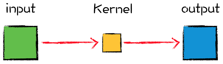
顺着示意图中箭头的方向,左侧是输入矩阵,中间是卷积核,右侧是输出矩阵。
标准卷积层
TensorFlow 框架里的标准卷积层的定义如下:
1 | tf.nn.conv2d( |
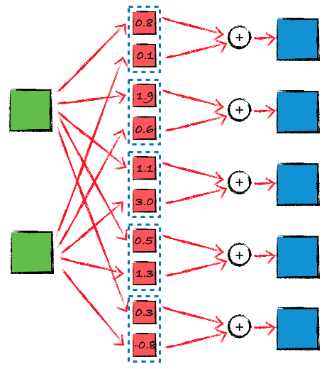
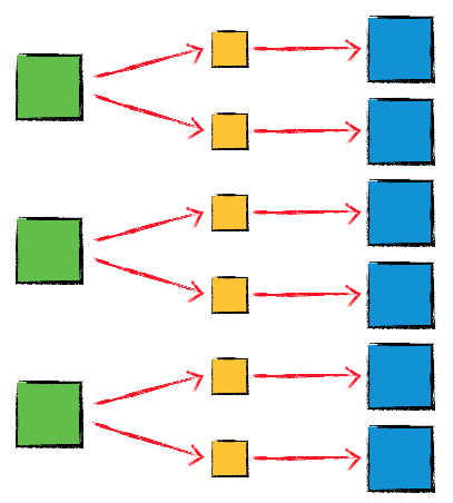
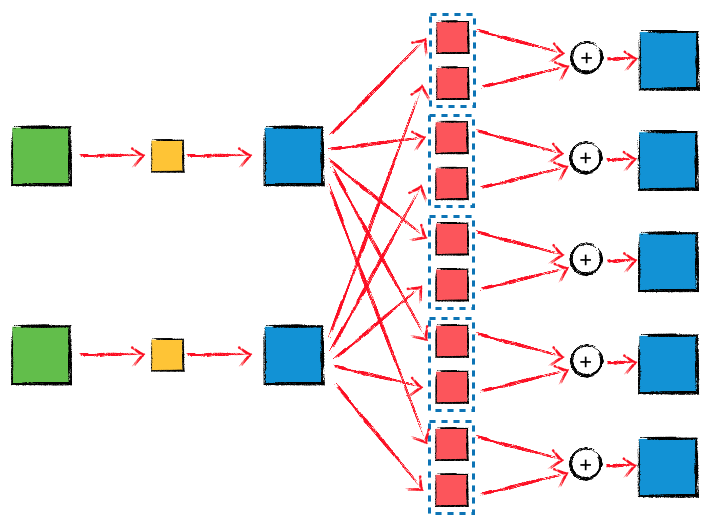
因为这里主要是为了讨论 channel 的映射规则,所以假设采用 ‘SAME’ padding,并且 strides 设置为 1,这样的话,输入的 Tensor 和 输出的 Tensor 中,height 和 width 都是相同的值,输入的 Tensor 的 shape 是 (batch_size, height, width, in_channels),如果期望的输出 Tensor 的 shape 是 (batch_size, height, width, out_channels),则作为 filter 的 Tensor 的 shape 应该设置成 (filter_height, filter_width, in_channels, out_channels),其中的 filter_height 和 filter_width 就对应卷积核的 size,这个函数内部的完整计算过程,可以用下面这个示意图来表示:
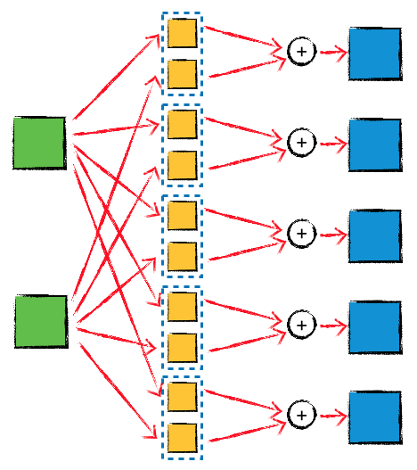
图中的 in_channels 等于 2,out_channels 等于 5,总共有 in_channels*out_channels = 10 个卷积核(同时还有 5 次矩阵加法操作),仔细看一下这个示意图就会意识到,每一个输出的矩阵都是由两个输入矩阵共同计算出来的,也就是说不同的输入 channel 会一起影响到每一个输出 channel,通道之间是有关联的。
One By One 卷积层
这种网络结构和前面介绍的标准卷积层其实是一样的,只不过 filter 的 shape 是 (1, 1, in_channels, out_channels),也就是说每一个卷积核都只是一个标量值,而非矩阵。表面上看这种结构有点违反『套路』,因为卷积的目的就是要利用周围像素的 加权和 来替代原始位置上的单个像素,或者说卷积每次关注的是一个区域的像素,而非只关注单个像素。
那 1x1 convolution 的目的是什么呢?前面已经提到了,神经网络里面的卷积层,既有卷积运算,也有 channel 之间的运算,所以 1x1 convolution 的重点就在于让不同的 channel 再结合一遍。类似的,也可以用一个简单的示意图表示这种网络结构:
1x1 convolution 的效果,相当于对输入矩阵做了一个简单的标量乘法,它的参数量和计算量都比标准的卷积层少了很多。前面 HED 代码里的 _output_1x1_conv2d 就是一个 1x1 convolution,在后面的讨论中也会遇到多个例子。
Depthwise 卷积层
标准卷积层运算,不同的输入 channel 会共同参与计算每一个输出 channel,还有另外一种名为 depthwise convolution 的卷积层运算,channel 之间是完全独立的,TensorFlow 里面的定义如下:
1 | tf.nn.depthwise_conv2d( |
类似的,假设采用 ‘SAME’ padding,并且 strides 设置为 1,最后的三个参数使用默认值,这样的话,输入 Tensor 和 输出 Tensor 的 height 和 width 就会是相同的值,输入的 Tensor 的 shape 是 (batch_size, height, width, in_channels),filter Tensor 的 shape 是 (filter_height, filter_width, in_channels, channel_multiplier),则得到的输出 Tensor 的 shape 是 (batch_size, height, width, in_channels * channel_multiplier),这个函数内部的完整计算过程,可以用下面这个示意图来表示:
可以看到,输出 Tensor 的 channels 不能是任意值,只能是 in_channels 的整数倍,这也就是参数 channel_multiplier 的含义。
Separable 卷积层
depthwise convolution 中,channel 之间是完全不会产生互相影响的,这可能也意味着这种方式的模型的复杂度是不够的,所以在实际使用的过程中,separable convolution 是一个更合适的选择,对应的 TensorFlow API 如下:
1 | tf.nn.separable_conv2d( |
同样的,采用 ‘SAME’ padding,并且 strides 设置为 1,最后的三个参数使用默认值,这样的话,输入 Tensor 和 输出 Tensor 的 height 和 width 就会是相同的值。这个 API 的内部首先执行了一次 depthwise convolution,然后执行了一次 1x1 convolution(pointwise convolution),所以 depthwise_filter 的 shape 应该设置为 (filter_height, filter_width, in_channels, channel_multiplier),pointwise_filter 的 shape 应该设置为 (1, 1, channel_multiplier * in_channels, out_channels),示意图如下:
在使用相同的 in_channels 和 out_channels 参数时,tf.nn.separable_conv2d 的运算量会比 tf.nn.conv2d 更小。
Dilated Convolutions / Atrous Convolution / 扩张卷积 / 空洞卷积
前面看到的几种不同的卷积层函数里,可能会有一个参数 rate,如果设置了 rate 并且 rate > 1,则内部执行了另外一种名为 Dilated Convolutions 的卷积运算操作,这种卷积运算的动画示意图如下:
在做边缘检测任务的时候,并没有用到 Dilated Convolutions,但是这种卷积操作也是很常用的,比如在 DeepLab 网络结构的各个版本中,它都是一个很重要的组件,考虑到这篇文章里已经汇总了多种不同的常用卷积操作,出于完整性的考虑,所以也简单提及一下 Atrous Convolution,有兴趣的同学可以进一步深入了解。
转置卷积/反卷积的初始化
HED 网络中是会用到转置卷积层的,简单回忆一下,transposed convolution 的动画示意图如下:
前一篇文章里提到过,当时是使用了双线性放大矩阵(bilinear upsampling kernel)来对反卷积的 kernel 进行的初始化,因为 FCN 要求采用这种初始化方案(HED 的论文中并没有明确的要求使用双线性初始化)。这次重写代码的时候,转置卷积层也统一替换成了 Xavier initialization,仍然能够得到很好的训练效果,同时也严格参照了 HED 的参考代码对转置卷积层的 kernel size 进行设置,具体的参数都在前面的函数 _dsn_deconv2d_with_upsample_factor 里面。
如何初始化 transposed convolution 的卷积核,这个问题其实纠结了很长时间,而且在前一个版本的 HED 的代码中,也尝试过用 tf.truncated_normal 初始化 transposed convolution 的 kernel,当时的确是没有训练出想要的效果,所以有点迷信『双线性初始化』,后来在做 UNet 网络的时候,因为已经接触到 Xavier initialization 方案了,所以也尝试了用 Xavier 对反卷积的 kernel 进行初始化,得到的效果很好,所以才开始慢慢的不再强求于『双线性初始化』。
Google 了很多文章,仍然没有找到关于『双线性初始化』的权威解释,只是找到过一些零星的线索,比如有些模型里,会把 deconvolution 的 kernel 的 learning rate 设置为 0,同时采用双线性插值矩阵对该 kernel 进行初始化,相当于就是通过双线性插值算法对输入矩阵进行上采样(放大)。目前我个人的准则就是,除非论文中有明确的强调要采用某种特殊的初始化方法,否则还是首先使用常规的 Tensor 初始化方案。这篇文章的读者朋友们,如果对这个问题有更清晰的答案,也请指教一下,谢谢~
顺便再举个例子,Deconvolution and Checkerboard Artifacts 这里就是用 resize-convolution 替代了常规的 deconvolution。
从 VGG 到 ResNet、Inception、Xception
前面着重介绍了几种不同的卷积层运算方式,目的就是为了引出这篇文章 An Intuitive Guide to Deep Network Architectures。VGG 作为一个经典的分类网络模型,它的结构其实是很简单的,就是标准卷积层串联在一起,如果想进一步提高 VGG 网络的准确率,一个比较直观的想法就是串联更多的标准卷积层(让网络变得更深)、在每一层里增加更多的卷积核,想法看上去是对的,但是实际的效果很不好,因为这种方式增加了大量的参数,训练起来自然就更难,而且网络的深度加深后,还会引起一个 梯度消失 的问题,所以简单粗暴并不总是有效的,需要想其他的办法。前面给出链接的这篇文章里介绍的三个重要网络结构,ResNet、Inception 和 Xception,就是为了解决这些问题而发展起来的,这三种网络模型使用的 层结构,已经成为了卷积神经网络领域里面的基础技术手段。
关于 ResNet、Inception、Xception 的详细内容,刚才提到的这篇文章就是一个很好的总结,网上也有一份整理过的中文翻译 无需数学背景,读懂 ResNet、Inception 和 Xception 三大变革性架构,在文末的参考资料里面还会列出几篇很棒的文章或代码。
如果是我自己对这三种网络结构做一个简单的总结,我觉得主要是下面几点:
- ResNet(残差网络) 使得训练更深的网络成为一种可能,既然很深的映射关系 Y = F(X) 不容易训练,那就改成训练 Y = F(X) + X,梯度消失问题就不再是一个障碍。
- Inception 架构通过增加每一层网络的宽度(使用不同 size 的卷积核,按照卷积核的大小进行分组)来提高网络的准确性,同时为了控制整体的运算量,借助 1x1 convolution 先对每一层的输入 Tensor 进行一个降维操作,减少 input channel 的数量,然后再进入每一个分组,用不同大小的卷积核进行计算。
- 残差架构可以和分组策略结合,比如 Inception-ResNet 网络结构。
- Inception 里面分组的概念使用到极致,就是让每一个通道成为一个独立的分组,在每个 channel 上先分别进行标准的卷积运算,然后再利用 1x1 convolution 得到最终的输出 channel,就其实就是 separable convolution。
从 MobileNet V1 到 MobileNet V2
ResNet、Inception、Xception 追求的目标,就是在达到更高的准确率的前提下,尽量在模型大小、模型运算速度、模型训练速度这几个指标之间找一个平衡点,如果在准确性上允许一定的损失,但是追求更小的模型和更快的速度,这就直接催生了 MobileNet 或类似的以手机端或嵌入式端为运行环境的网络结构的出现。
MobileNet V1 和 MobileNet V2 都是基于 Depthwise Separable Convolution 构建的卷积层(类似 Xception,但是并不是和 Xception 使用的 Separable Convolution 完全一致),这是它满足体积小、速度快的一个关键因素,另外就是精心设计和试验调优出来的层结构,下面就对照论文给出两个版本的代码实现。
MobileNet V1
MobileNet V1 的整体结构其实并没有特别复杂的地方,和 VGG 类似,层和层之间就是普通的串联型的结构,有区别的地方主要在于 layer 的内部,如下图所示:
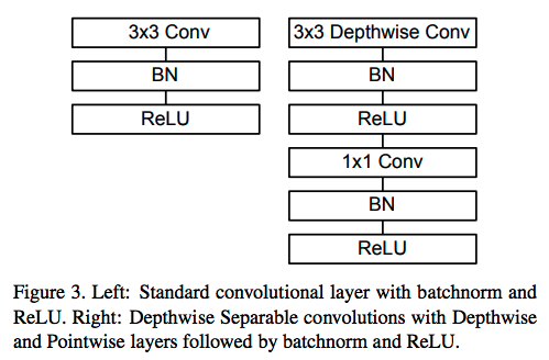
这个图中没有用箭头表示数据的传递方向,但是只要对卷积神经网络有初步的经验,就能看出来数据是从上往下传递的,左图是标准的卷积层操作,类似于前面 HED 网络中 _vgg_conv2d 函数的结构(回想一下前面说过的 Batch Normalization 和 relu 先后顺序的话题,虽然 Batch Normalization 可以放到激活函数的后面,但是很多论文里面都还是习惯性的放在激活函数的前面,所以这里的代码也会严格的遵照论文中的方式),右侧的图相当于 separable convolution,但是在中间是有两次 Batch Normalization 的。
论文中用一张如下的表格来描述了整体结构:
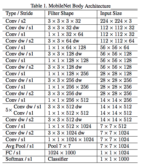
下面是一份简单的代码实现:
1 | def mobilenet_v1(inputs, alpha, is_training): |
MobileNet V2
MobileNet V2 的改动就比较大了,首先引入了两种新的 layer 结构,如下图所示:
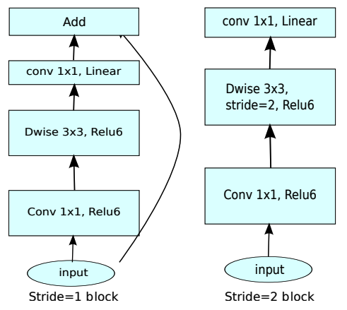
很明显的一个差异点,就是左边这种层结构引入了残差网络的手段,另外,这两种层结构中,在 depthwise convolution 之前又添加了一个 1x1 convolution 操作,在之前举得几个例子中,1x1 convolution 都是用来降维的,而在 MobileNet V2 里,这个位于 depthwise convolution 之前的 1x1 convolution 其实用来提升维度的,对应论文中 expansion factor 参数的含义,在 depthwise convolution 之后仍然还有一次 1x1 convolution 调用,但是这个 1x1 convolution 并不会跟随一个激活函数,只是一次线性变换,所以这里也不叫做 pointwise convolution,而是对应论文中的 1x1 projection convolution。
网络的整体结构由下面的表格描述:
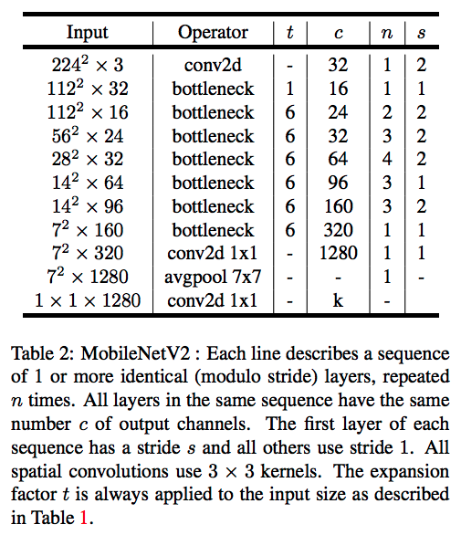
代码实现如下:
1 | def mobilenet_v2_func_blocks(is_training): |
MobileNet V2 Style HED
原始的 HED 使用 VGG 作为基础网络结构来得到 feature maps,参照这种思路,可以把基础网络部分替换为 MobileNet V2,代码如下:
1 | def mobilenet_v2_style_hed(inputs, batch_size, is_training): |
这个 MobileNet V2 风格的 HED 网络,整体结构和 VGG 风格的 HED 并没有区别,只是把 VGG 里面用到的卷积层操作替换成了 MobileNet V2 对应的卷积层,另外,因为 MobileNet V2 的第一个卷积层就设置了 stride=2,并不匹配 dsn1 层的 size,所以额外添加了两个 stride=1 的普通卷积层,把它们的输出作为 dsn1 层。
MobileNet V2 As Base Net
MobileNet 只是针对手机运行环境设计出来的执行 分类任务 的网络结构,但是,和同样执行分类任务的 ResNet、Inception、Xception 这一类网络结构类似,都可以作为执行其他任务的网络结构的 base net,提取输入 image 的 feature maps,我尝试过 mobilenet_v2_style_unet、mobilenet_v2_style_deeplab_v3plus、mobilenet_v2_style_ssd,都是可以看到效果的。
Android 性能瓶颈
作为一个参考值,在 iPhone 7 Plus 上运行这个 mobilenet_v2_style_hed 网络并且执行后续的找点算法,FPS 可以跑到12,基本满足实时性的需求。但是当尝试在 Android 上部署的时候,即便是在高价位高配置的机型上,FPS 也很低,卡顿现象很明显。
经过排查,找到了一些线索。在 iPhone 7 Plus 上,计算量的分布如下图所示:
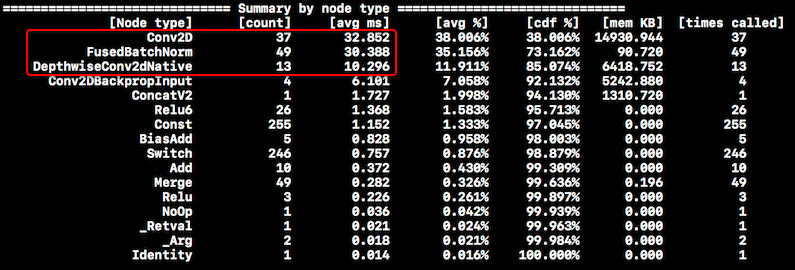
红框中的三种操作占据了大部分的 CPU 时间,用这几个数值做一个粗略估算,1.0 / (32 + 30 + 10 + 6) = 12.8,这和检测到的 FPS 是比较吻合的,说明大量的计算时间都用在神经网络上了,OpenCV 实现的找点算法的耗时是很短的。
但是在 Android 上,情况则完全不一样了,如下图所示:
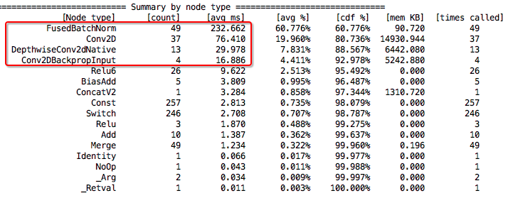
用红框里的数值计算一下,FPS = 1.0 / (232 + 76 + 29 + 16) = 2.8,达不到实时的要求。从上图还可以看出,在 Android 上,Batch Normalization 消耗了大量的计算时间,而且和 Conv2D 消耗的 CPU 时间相比,不在一个数量级上了,这就和 iOS 平台上完全不是同一种分布规律了。进一步 debug 后发现,我们 Android 平台的 app,由于一些历史原因被限定住了只能使用 32bit 的 .so 动态库,换成 64bit 的 TensorFlow 动态库在独立的 demo app 里面重新测量,mobilenet_v2_style_hed 在 Android 上的运行情况就和 iOS 的接近了,虽然还是比 iOS 慢,但是 CPU 耗时的统计数据是同一种分布规律了。
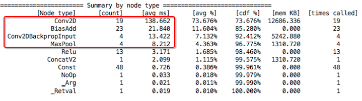
所以,性能瓶颈就在于 Batch Normalization 在 32bit 的 ARM CPU 环境中执行效率不高,尝试过使用一些编译器优化选项重新编译 32bit 的 TensorFlow 库,但是并没有明显的改善。最后的解决方案是退而求其次,使用 vgg_style_hed,并且不使用 Batch Normalization,经过这样的调整后,Android 上的统计数据如下图:
关于 TensorFlow Lite
在使用 TensorFlow 1.7 部署模型的时候,TensorFlow Lite 还未支持 transposed convolution,所以没有使用 TF Lite (目前 github 上已经看到有 Lite 版本的 transpose_conv.cc 了)。TensorFlow Lite 目前发展的很快,以后在选择部署方案的时候,TensorFlow Lite 是优先于 TensorFlow Mobile 的。
参考资料
xavier init
How to do Xavier initialization on TensorFlow
聊一聊深度学习的weight initialization
Batch Normalization
Understanding the backward pass through Batch Normalization Layer
机器学习里的黑色艺术:normalization, standardization, regularization
How could I use Batch Normalization in TensorFlow?
add Batch Normalization immediately before non-linearity or after in Keras?
1x1 Convolution
What does 1x1 convolution mean in a neural network?
How are 1x1 convolutions the same as a fully connected layer?
One by One [ 1 x 1 ] Convolution - counter-intuitively useful
Upsampling && Transposed Convolution
Upsampling and Image Segmentation with Tensorflow and TF-Slim
Image Segmentation using deconvolution layer in Tensorflow
ResNet && Inception && Xception
Network In Network architecture: The beginning of Inception
ResNets, HighwayNets, and DenseNets, Oh My!
Inception modules: explained and implemented
TensorFlow implementation of the Xception Model by François Chollet